A Few Minutes on the Pesticide Paradox

Source: Orhan Akbaba on Pexels

One of the first assignments of my MSc was to present a topic to my peers. We were given an optional list of topics to choose from or we could pick one of our own. I trusted the instincts of the module leader, knowing that if I stray too far out of the range of the prescribed topics, I could see myself waffling and sending my peers to sleep. Some of the predetermined topics were as follows:

• The four-colour theorem
• The Black-Scholes option pricing model
• Dorfman’s algorithm for combinatorial group testing
• Penrose’s aperiodic tilings of the plane
• The twin prime conjecture
• The chaos game
• The Lotka-Volterra predator-prey equations
• Recurrence and transience of random walks
• The contraction mapping theorem.

I have always enjoyed visualising maths, and I had very much enjoyed learning about dynamical systems, so the Lotka-Volterra equations seemed a good choice. One issue arose, however: How could I explore the Lotka-Volterra equations in five minutes whilst making it somewhat interesting? Of course, one would expect the average MSc Mathematics student to know what they are or to have at least heard of them; I didn’t want to merely relay information that my peers are familiar with - that seemed boring to me. For those unfamiliar, the Lotka-Volterra equations show how the population densities of two species, \(x\) and \(y\), change with time:

\[\begin{aligned} \frac{\mathrm{d}x}{\mathrm{d}t} &= \alpha x - \beta xy \\ \\ \frac{\mathrm{d}y}{\mathrm{d}t} &= -\gamma y + \delta xy \end{aligned}\]

where \(\alpha\), \(\beta\), \(\gamma\), and \(\delta\) are positive constants which represent the interactive behaviour between the two species.

Fortunately, a quick Google search of the Lotka-Volterra equations revealed discussions around the Paradox of the Pesticides; a consequence of applying pesticide to a two-species system of Lotka-Volterra equations. This was my answer - an interesting look at the L-V equations which all of my peers could access and from which learn something new (hopefully).

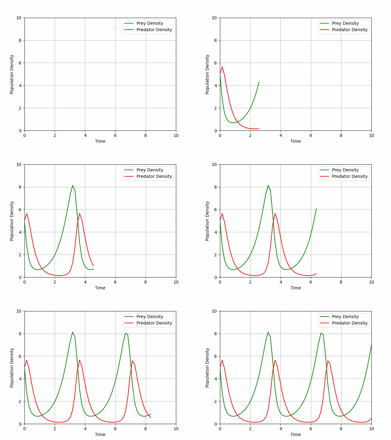
So, I began to plan out my presentation. A definition of the Lotka-Volterra equations followed by an exposition of what happens mathematically when one introduces pesticide to the system. In order to do this, I produced animations using Python to demonstrate how the population densities dictated by a stable Lotka-Volterra system fluctuate with time (see Figure 1).

Figure 1: A stable predator-prey system described by the Lotka-Volterra equations. Source: Self-produced using Python.

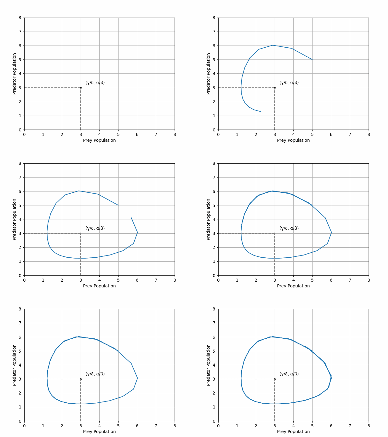
Another way of visualising the prey density dynamics is by plotting the densities against each other, revealing a circular orbit for a stable system centred at its non-trivial fixed point (see Figure 2).

Figure 2: A prey density - predator density plot to illustrate the stability of the system. Source: Self-produced using Python.

Now, let’s discuss the impact of adding pesticide to this system. In the context of this paradox, we assume that the pesticide is a linear term introduced to both equations as follows:

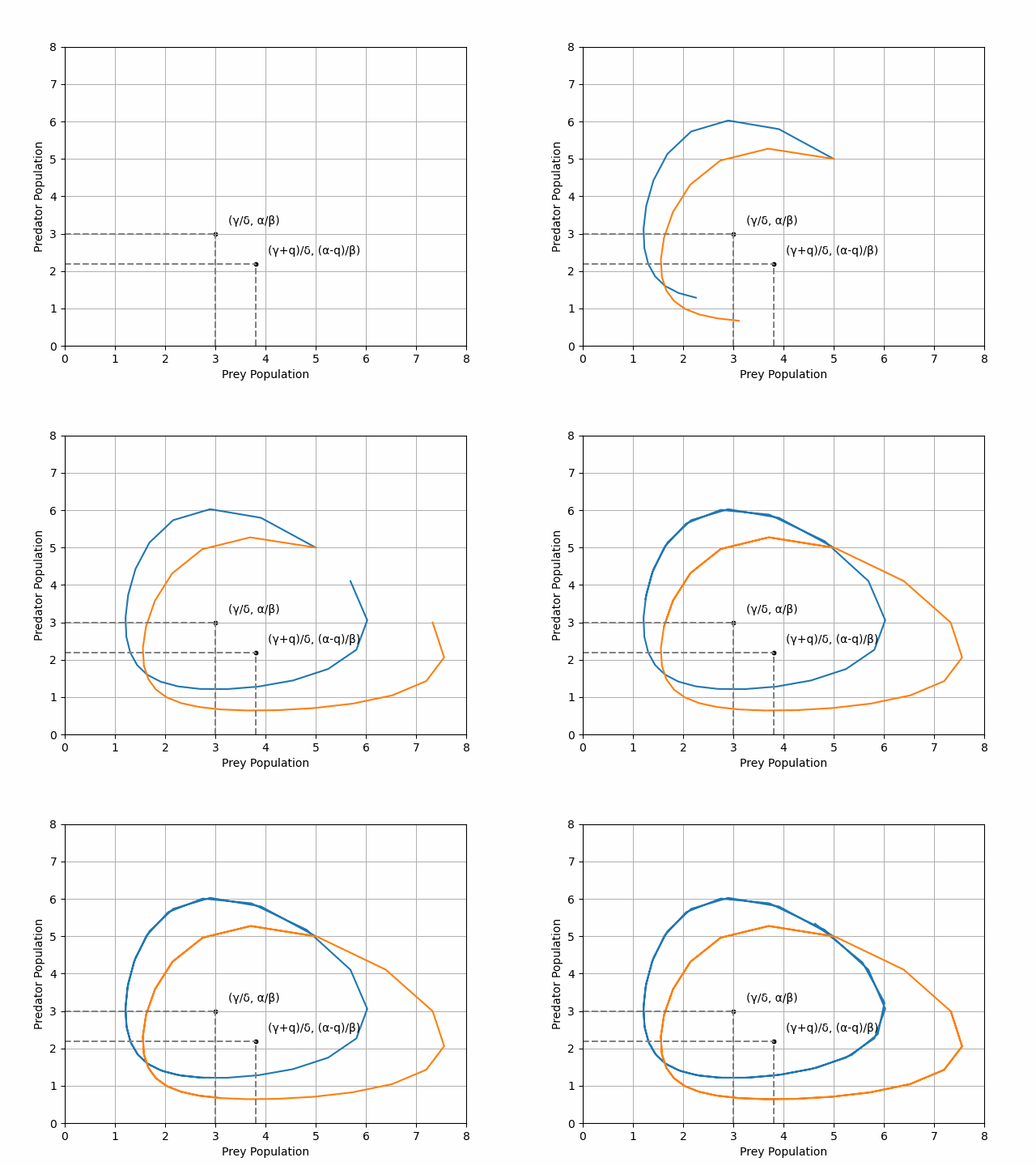
\[\begin{aligned} \frac{\mathrm{d}x}{\mathrm{d}t} &= \alpha x - \beta xy - qx \\ \\ \frac{\mathrm{d}y}{\mathrm{d}t} &= -\gamma y + \delta xy -qy \end{aligned}\]

where \(q\) denotes the impact of the pesticide on both prey and predator densities. Plotting the trajectory of our new equations, combined with the trajectory of the original unpeturbed Lotka-Volterra equations reveals a paradoxical result (see Figure 3).

Figure 3: A comparison of the unperturbed system and the peturbed system to demonstrate the impact of adding pesticide to the Lotka-Volterra system. Source: Self-produced using Python.

We see that the pesticide-ladened system has (on average) a higher density of prey! We had hoped to reduce the prey density by adding pesticide but have in fact increased it.

A fascinating result explored in five minutes.

Thanks for reading! Please see the LaTex/Beamer presentation here (you may have to use Adobe Acrobat to view the animations within the Beamer presentation).