Randomly Walking in Python, Stylishly

Source: Marshall, using Python

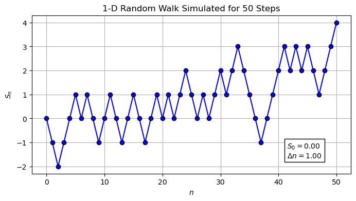
When learning about stochastic processes, we are often first introduced to the simple, symmetric random walk. In this post, I show how one can produce a plot of a random walk in Python and the various methods you can implement to make it look a little nicer.

Firstly, please see below the mathematical definition of a simple, symmetric random walk:

Definition 1: Simple Random Walk

Let \(\left\{X_i\right\} \sim \text{Be}(0.5)\) for \(i \in \mathbb{N}\) be a set of independent and identically distributed (i.i.d.) random variables, each taking either the value 1 or -1. Then, a simple symmetric random walk, \(S_n\), of \(n \in \mathbb{N}\) steps, is an iterative process given by
\(S_{n+1} = S_n + X_n\)
where \(S_0=0\) denotes the initial starting point.

Rather handwavingly, one may think of a simple symmetric random walk as a walker stepping forward by one metre or backwards by one metre with equal probability for each step of their walk. Flip a coin: heads is forwards, tails is backwards. After \(n\) flips, your displacement from your initial point is given by \(S_n\).

One may of course generalise this by changing the step size from one metre and by changing the probability of stepping forward each step to be a value other than one-half. However, this is outside the scope of this post. We will instead focus on how to plot a simple symmetric random walk in Python.

Let’s start with the basics; we shall first implement our above definition in Python:

# Imported libraries:
import matplotlib.pyplot as plt # # matplotlib enables us to produce and customise many of the plots visible throughout the code.  
import numpy as np # NumPy is a library which contains multiple methods required for data manipulation, particularly when working with arrays.

number_of_steps = 5 # How many steps does the random walk take. In this case, it is five. 
x = np.zeros(number_of_steps) # This creates an array of zeros to store the value of the random walk.

for i in range(1, number_of_steps): # For each step...
    step = np.random.choice([-1, 1])  # This chooses either 1 or -1 with equal probability
    x[i] = x[i-1] + step # This calculates the displacement of the random walk at time i.

print(x)

This will return an array, \(x\), of the values after each step of the random walk. In my case, this returned an \(x\) array of:

[ 0 -1 -2 -1 -2 ]

This means that the walk starts at 0, then moves to -1 in the second step, then to -2, then to -1, then to -2. Notice that each step either increases or decreases by 1.

Let’s now take a look at how to plot it!

# Imported libraries:
import matplotlib.pyplot as plt # matplotlib enables us to produce and customise many of the plots visible throughout the code.  

plt.plot( x,               # This first argument is the thing we want to plot.
          marker='o',      # The second argument specifies the shape of each data point.
          mec = 'black',   # The third argument gives a nice outline around the marker
          linestyle='-')   # Linestyle allows you to specify whether you want a dashed line or not.
    
plt.title('Simple Random Walk') # Provides a title
plt.xlabel('Step') # Labels x-axis
plt.ylabel('Position') # Labels y-axis
plt.grid()   # This creates a set of gridlines on our plot.

Here is my output below:

If you wish to save your image in Python, append your code with a line stating:

plt.savefig('random_walk_image.png')

Pretty cool, eh?

References

• P. R´ev´esz. Random walk in random and non-random environments. World Scientific, 2013.