1.0 What are networks? (nodes and edges)
Networks are used to describe many real-world phenomena such as the interaction within social structures and the mapping of transport links connecting cities. In this post, we shall introduce the fundamental concepts of network theory.
Nodes and edges
In the same way that we can portray a function with a plot, we can model a network with a graph. A graph is made up of nodes connected by edges. The following example will motivate understanding here.
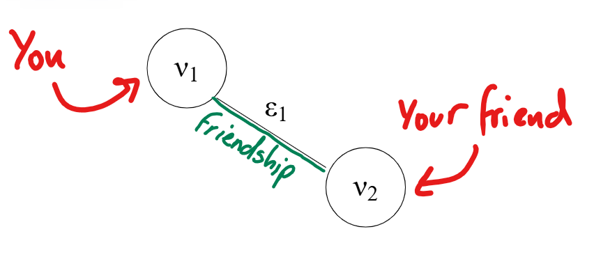
We can create a graph of the network between you and a friend; there are two nodes (you and your friend) connected by an edge (a straight line representing your friendship):

It is customary to call nodes \(\nu\) with a subscript to differentiate between each node. You can see here that ‘you’ are labelled \(\nu_1\) and ‘your friend’ is represented as \(\nu_2\). The edge connecting them is denoted by \(\epsilon_1\), following the same subscript rules as our nodes.
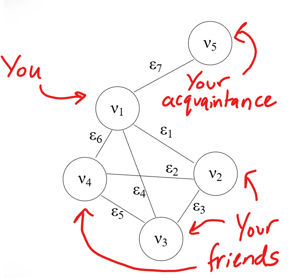
A graph can consist of more than one node, you may wish to construct a network between you, your friend group, and an acquaintance of yours.

The set of nodes \(\nu\), in this example, is given by:
\(\begin{equation} \nu = \left\{ \nu_1, \nu_2, \nu_3, \nu_4, \nu_5 \right\} \end{equation}\).
The set of edges \(\epsilon\), in this example is given by:
\[\begin{align} \epsilon &= \begin{cases} \epsilon_1 = (\nu_1, \nu_2), \\ \epsilon_2 = (\nu_2, \nu_4), \\ \epsilon_3 = (\nu_2, \nu_3), \\ \epsilon_4 = (\nu_1, \nu_3), \\ \epsilon_5 = (\nu_3, \nu_4), \\ \epsilon_6 = (\nu_1, \nu_4), \\ \epsilon_7 = (\nu_1, \nu_5) \end{cases} \end{align}\]Now we have this intuition, let’s define a simple, undirected graph.
Definition 1: Undirected Graph
An undirected network is a set of nodes, \(\nu = \{\nu_1, \nu_2, \ldots, \nu_N\}\), and a set of edges, \(\epsilon = \{\epsilon_1, \epsilon_2, \ldots, \epsilon_K\}\), for \(K, N \in \mathbb{N}\) such that each edge in \(\epsilon\) connects an element in \(\nu\) to another (not necessarily distinct) element of \(\nu\).
This definition implies there is a directed graph. In fact, our edges can be directed in a single direction.
However, for the rest of this post, we will consider undirected graphs. I may create a future post on directed graphs at a later date.
It is almost always important to consider the connectivity of nodes. This is where the real magic of networks reveals itself. Fortunately, there is a super legible way to convey the interconnectivity of nodes - this is known as the adjacency matrix.
Adjacency matrix
The adjacency matrix tells us what nodes are connected to each node in a legible format.
Definition 2: Adjacency Matrix
Given an undirected network (as in Definition 1), the adjacency matrix, \(A\), is defined as a symmetric \(N \times N\) matrix where:
\[\begin{equation} A_{ij} = \begin{cases} 1 & \text{if } (i, j) \in \epsilon \\ 0 & \text{if } (i, j) \notin \epsilon \end{cases} \end{equation}\]for integers \(i, j \in \left\{1, \ldots, N \right\}\)
From this definition, one can see that there is a \(1\) in the \(ij\)-th element of the adjacency matrix if nodes \(\nu_i\) and \(\nu_j\) are connected.
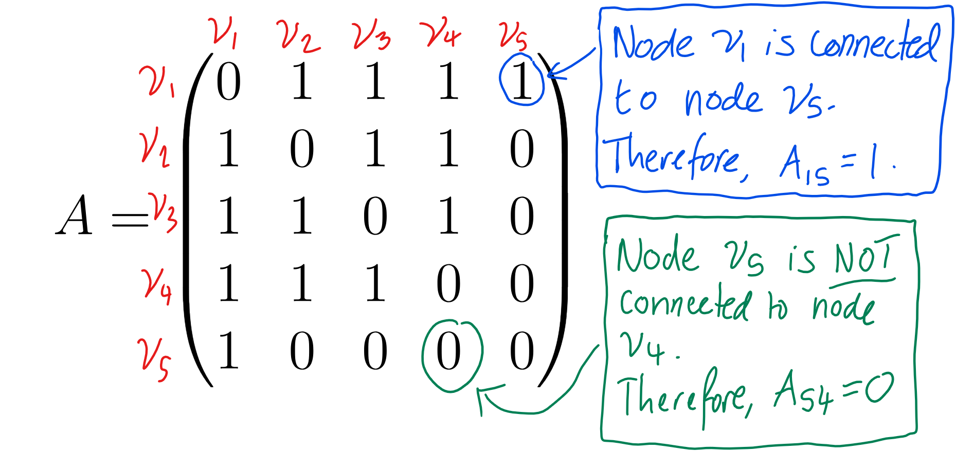
As an example, consider the graph in Figure 2. One can create its adjacency matrix:
\[A = \begin{pmatrix} 0 & 1 & 1 & 1 & 1 \\ 1 & 0 & 1 & 1 & 0 \\ 1 & 1 & 0 & 1 & 0 \\ 1 & 1 & 1 & 0 & 0 \\ 1 & 0 & 0 & 0 & 0 \\ \end{pmatrix}\]To see this a bit more clearly, I have annotated which node is connected to each node by labelling the rows and columns of the above adjacency matrix.

As you can see, in congruence with Figure 2, everybody knows everybody in your friend group, and your acquaintance is only known by you. The adjacency matrix allows us to represent the connectivity of a given network without having to draw the graph. It is easy to imagine that drawing a graph with a large number of nodes and/or edges can become quite a headache.
Incidence matrix
We may wish to consider the connectivity of a graph from the perspective of its edges. This is known as the incidence matrix; a way of capturing how each node is incident (connected) to each edge.
Definition 3: Incidence Matrix
Given an undirected network (as in Definition 1), the incidence matrix, \(E\), is defined as an \(N \times K\) matrix where:
\[\begin{equation} E_{ij} = \begin{cases} 1 \text{ if } \nu_i \in \epsilon_j\\ 0 \text{ if } \nu_i \notin \epsilon_j\ \end{cases} \end{equation}\]for integers \(i \in \left\{1, \ldots, N \right\}\) and \(j \in \left\{1, \ldots, K \right\}\)
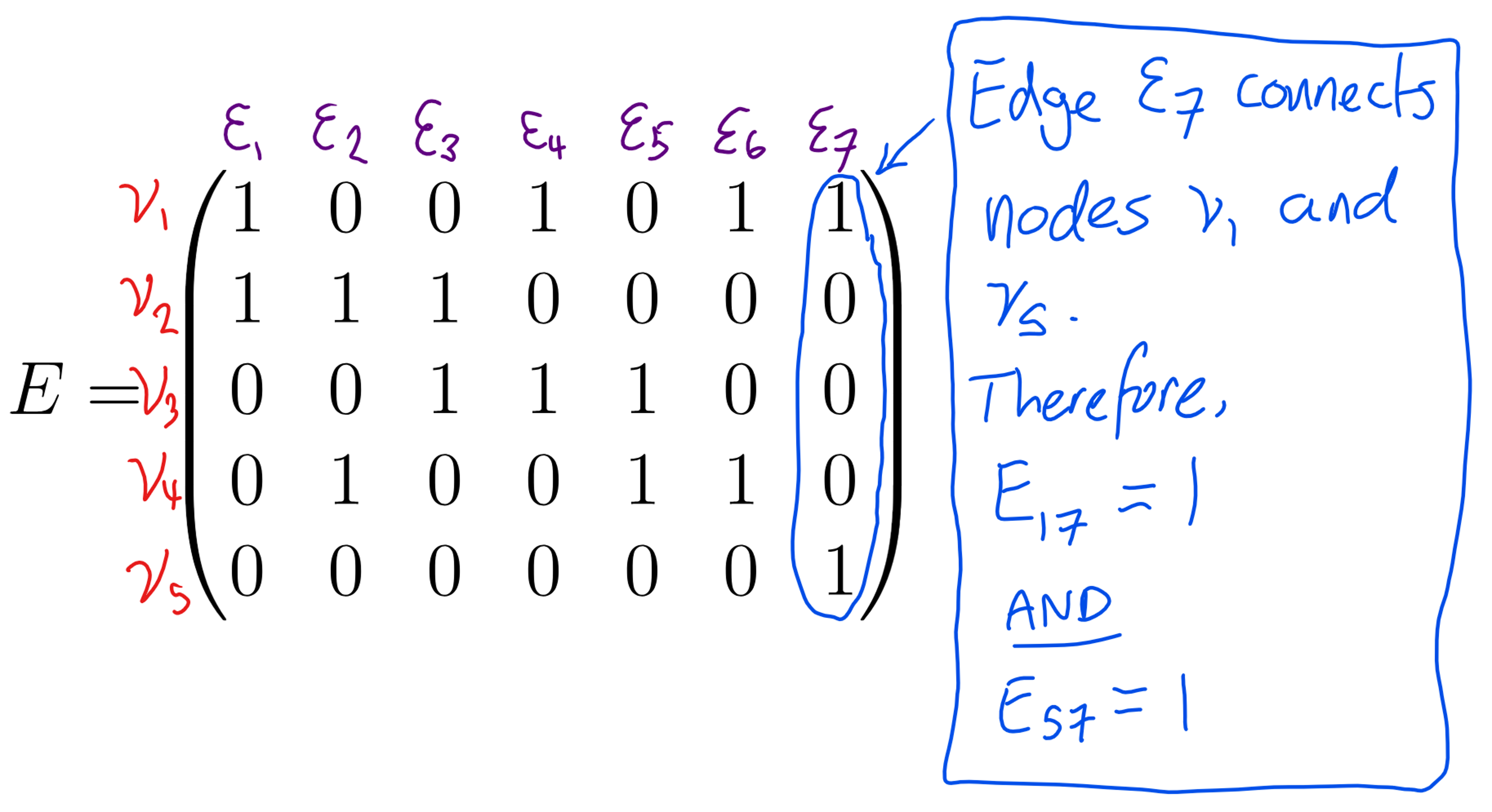
If we consider the graph in Figure 2, one can create its incidence matrix:
\[E = \begin{pmatrix} 1 & 0 & 0 & 1& 0 & 1& 1 \\ 1 & 1 & 1 & 0& 0 & 0 & 0\\ 0 & 0 & 1 & 1& 1 & 0 & 0\\ 0 & 1 & 0 & 0& 1 & 1 & 0\\ 0 & 0& 0 & 0& 0 & 0 & 1\\ \end{pmatrix}\]To see this a bit more clearly, I have annotated which edge is incident to each node by labelling the columns and rows respectively.

This is an alternative way to portray the connectivity of the network and becomes very useful if your focus is on the edges between specific units. In transport networks, the edges are often the primary focal points of investigation.
Node degree
Another important measure of connectivity is the node degree of a given node within a network. A formal definition of the node degree can be found below.
Definition 4: Node Degree
Given an undirected network, \(G = \left\{ \nu, \epsilon \right\}\), with $N$ nodes (as in Definition 1), the node degree of a given node \(\nu_i\) can be defined by the adjacency matrix:
\[\begin{equation} \text{deg}(\nu_i) = \sum_{j = 1}^{N} A_{ij} \end{equation}\]for integer \(i \in \left\{1, \ldots, N \right\}\)
One can think of the node degree as the number of connections that the node in question has. This can be a useful quantifier of a person’s popularity or a measure of how accessible an area is by transport links.
In the network portrayed in Figure 2, we can count the node degree by either using the adjacency matrix or by counting how many edges are attached to each node. Check that you can do this by confirming my results below with the graph in Figure 2:
\[\begin{align}\text{deg}(\nu_1) &= A_{11} + A_{12} + A_{13} + A_{14} + A_{15} \\ &= 0 + 1 + 1 + 1 + 1 \\ &= 4 \end{align}\] \[\begin{align}\text{deg}(\nu_2) &= A_{21} + A_{22} + A_{23} + A_{24} + A_{25} \\ &= 1 + 0 + 1 + 1 + 0 \\ &= 3 \end{align}\] \[\begin{align}\text{deg}(\nu_3) &= A_{31} + A_{32} + A_{33} + A_{34} + A_{35} \\ &= 1 + 1 + 0 + 1 + 0 \\ &= 3 \end{align}\] \[\begin{align}\text{deg}(\nu_4) &= A_{41} + A_{42} + A_{43} + A_{44} + A_{45} \\ &= 1 + 1 + 1 + 0 + 0 \\ &= 3 \end{align}\] \[\begin{align}\text{deg}(\nu_5) &= A_{51} + A_{52} + A_{53} + A_{54} + A_{55} \\ &= 1 + 0 + 0 + 0 + 0 \\ &= 1 \end{align}\]This tells us that node \(\nu_1\) has the highest node degree and is therefore the most connected node in this network. In the next section, we will discuss what we can do with this information to infer global properties of the network.
Node degree distribution
When looking at the global properties of networks, we often like to determine the node degree of each node within our network. It is then convenient for us to determine the probability distribution of node degrees (i.e., the probability of choosing a node with degree \(k\) out of all possible nodes \(N\)). Please see a formal definition of this distribution below:
Definition 5: Node Degree Distribution
Given an undirected network, \(G = \left\{ \nu, \epsilon \right\}\), with \(N\) nodes (as in Definition 1), the node degree distribution is a probability distribution, \(P(k)\), such that:
\[\begin{equation} P(k) = \frac{n_k}{N} \end{equation}\]where \(n_k\) is the number of nodes in the network with degree \(k\).
By counting the number of nodes with degree \(k\) and dividing by the total number of nodes, we are able to generate a discrete probability distribution for the node degree. Please see the node degree distribution for the network portrayed in Figure 2 below:
\[\begin{equation} P(k) = \begin{cases} \frac{1}{5} & \text{if } k = 1 \\ \frac{3}{5} & \text{if } k = 3 \\ \frac{1}{5} & \text{if } k = 4 \\ 0 & \text{ otherwise } \end{cases} \end{equation}\]It is customary to exclude the values of degree value \(k\) in the degree distribution for which there are no nodes present. Notice in our previous calculations that there was one node with degree one, three nodes with degree three, and one node with degree four. The node degree distribution is a probability distribution that encompasses the proportion of node degrees seen throughout the network.
