1.0 Simple Linear Regression

Imagine we have collected data on the amount of time students have studied for a test and their respective scores from that test. Simple linear regression allows us to model the relationship between time spent studying and test scores. The phrase simple linear regression is a bit of a mouthful, so let’s first break down its etymology:

• The term ‘regression’ was used by early statisticians working on data modelling to describe the moving trend of data with respect to the independent variable. It is stated that Francis Galton used the term to describe how heights of children regressed; he noticed that the children’s heights tended to “regress” towards the average height of the population, rather than staying as extreme as their parents’ height. Today, we use the term regression to describe the relationship between variables.
• The term ‘simple’ refers to the fact that we are (in this post) only dealing with one independent variable.
• The term ‘linear’ points to the linearity of the model, in that we wish to represent the relationship with a straight line. This will make more sense later.

Formally, we wish to model the set of observed values \(\left\{y_i\right\}\) (e.g., test scores) based on a set of values of an independent variable \(\left\{x_i\right\}\) (e.g., amount of time studied per student). The simple linear regression model may look like this:

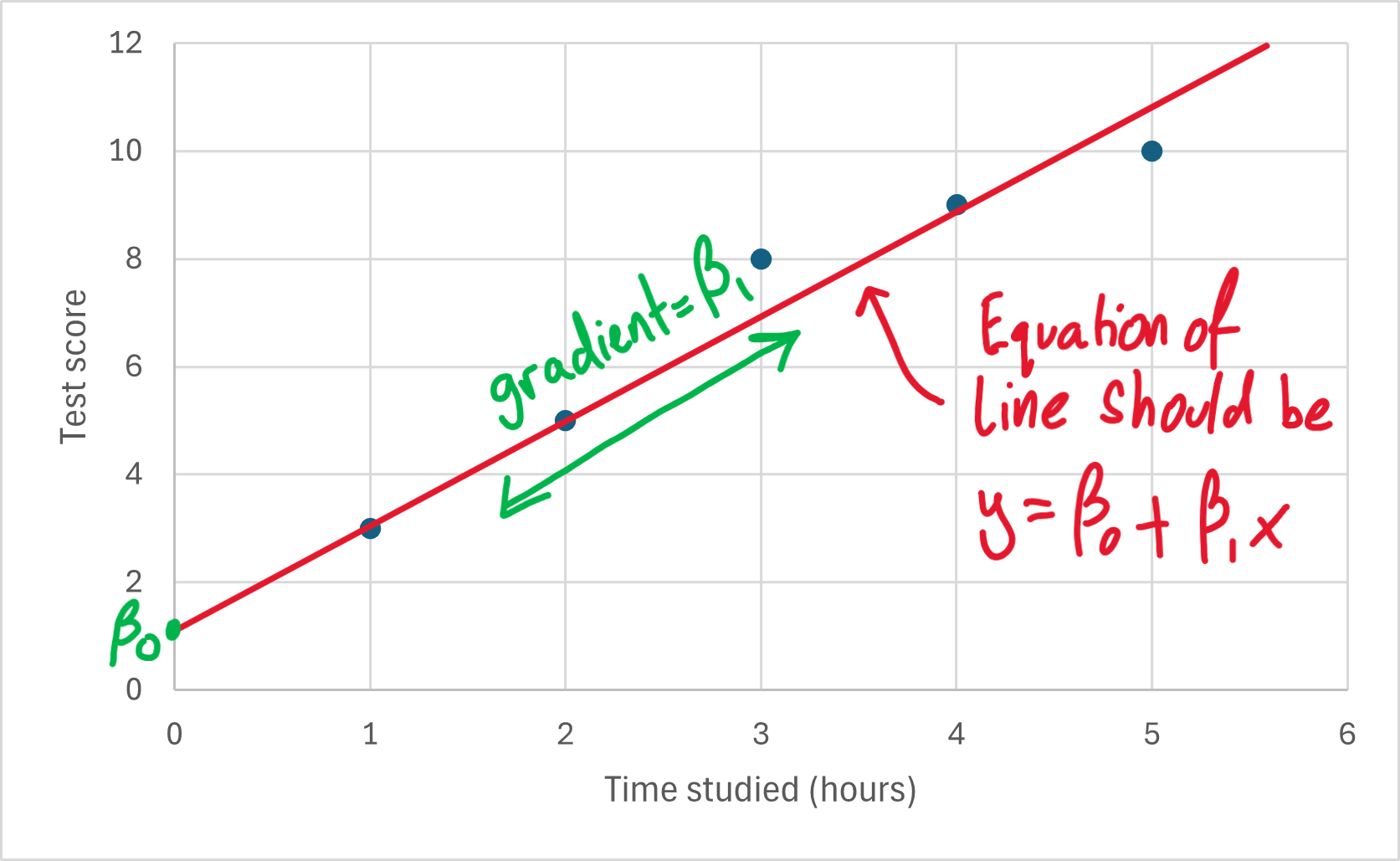
\[\begin{equation} y_i = \beta_0 + \beta_1 x_i + \epsilon_i \end{equation}\]

where \(\beta_0, \beta_1 \in \mathbb{R}\) are coefficients indicating the intercept and gradient of our straight line respectively. We also have an error term \(\epsilon_i \sim \mathcal{N}(0, \sigma^2)\) which accounts for the dispersion of the observed values about the straight line.

We interpret this model by recognising that a one-unit change in \(x_i\) will result in an approximate \(\beta_1\) increase in \(y_i\). To see this more clearly, we can write this model out fully for each \(y_i\) for \(i = 0, 1, 2, 3, \ldots, n\):

\[\begin{equation} y_1 = \beta_0 + \beta_1 x_1 + \epsilon_1 \end{equation}\] \[\begin{equation} y_2 = \beta_0 + \beta_1 x_2 + \epsilon_2 \end{equation}\] \[\begin{equation} y_3 = \beta_0 + \beta_1 x_3 + \epsilon_3 \end{equation}\] \[\begin{equation} \vdots \end{equation}\] \[\begin{equation} y_n = \beta_0 + \beta_1 x_n + \epsilon_n \end{equation}\]

From here, we can easily see that this model can be written as a matrix equation:

\[\begin{equation} \begin{pmatrix} y_1 \\ y_2 \\ y_3 \\ \vdots \\ y_n \end{pmatrix} = \begin{pmatrix} 1 & x_1 \\ 1 & x_2 \\ 1 & x_3 \\ \vdots & \vdots \\ 1 & x_n \end{pmatrix}\end{equation} \begin{pmatrix} \beta_0 \\ \beta_1 \\ \end{pmatrix} + \begin{pmatrix} \epsilon_1 \\ \epsilon_2 \\ \epsilon_3 \\ \vdots \\ \epsilon_n \end{pmatrix}\]

Or, more compactly:

\[\begin{equation} \underline{y} = \underline{\underline{F}} \underline{\beta} + \underline{\epsilon} \end{equation}\]

\(\underline{\underline{F}}\) is sometimes referred to as the design matrix. We shall use this nomenclature going forward.

Let’s now consider the meaning of this model and, more importantly, what it can tell us. One may imagine linear regression as a tool to plot a line of best fit between our set of independent variable values \(\left\{x_i\right\}\) and their respective responses \(\left\{y_i\right\}\). This can be illustrated by plotting a set of coordinates for each \(i = 0, 1, 2, 3, \ldots, n\).

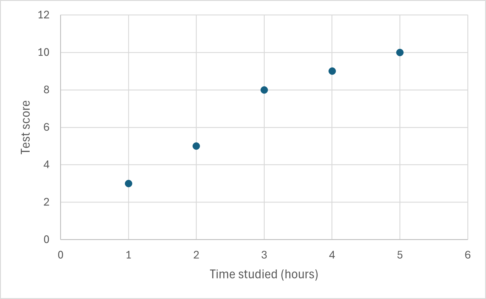
As an example, let us refer back to our time studied and test score investigation. After the test, I gathered the following results:

\[\begin{align} &x = \left\{1, 2, 3, 4, 5\right\} \ \leftarrow \texttt{hours studied} \\ &y = \left\{3, 5, 8, 9, 10\right\} \ \leftarrow \texttt{test scores} \end{align}\]

Let’s plot this on a scatter graph:

Figure 1: A scatter plot showing test scores and time studied for five students.

Below, I have annotated this chart to show the role of \(\beta_0\) and \(\beta_1\) in the line of best fit.

Figure 2: The above scatter graph, annotated.

However, how do I know what the “best” \(\beta_0\) and \(\beta_1\) are for this model?

The aim of simple linear regression is to find \(\beta_0\) and \(\beta_1\) such that our line of best fit indeed fits the relationship as best as possible. This notion forms the basis of our next post: Estimating \(\beta_0\) and \(\beta_1\) using something called least squares estimation. I will explain what this means in the next post - see you there! :)